Saturday, June 28, 2008

pedagogical moment: LaTeX, TeX, environments, and csname

On the MiKTeX mailing list, a thread descended into a flame that someone bracketed with \flameon and \flameoff, which is a sort of Fantastic Four version of a LaTeX environment. The thread involved the differences between TeX, Plain TeX, and LaTeX, and so I took the opportunity to point a few things out. I received several positive responses, and so I decided to reproduce my post here.
\pedagogical

There's a TeX vs. LaTeX teachable moment here . . .

> > \flameon
...
> > \flameoff


     As an example, if you're using LaTeX, the proper code for a flame environment is:
\begin{flame}
\end{flame}
However, the \begin and \end macros do nothing more than call:
\flame
\endflame
and so bracketing an environment in these macros is (in principle) equivalent to using the \begin and \end environments.

     Further, a naive implementation of \begin and \end is:
\newcommand\begin[1]{\csname #1\endcsname}
\newcommand\end[1]{\csname end#1\endcsname}
which is equivalent to the "raw" TeX (which may also be used in LaTeX):
\def\begin#1{\csname #1\endcsname}
\def\end#1{\csname end#1\endcsname}
In other words, \newcommand and \def are basically the same beast. However, \newcommand is a macro (created with \def) that checks to make sure you haven't already \newcommand'd before. SIMILARLY, the REAL \begin and \end wrappers have extra sanity checks for safety.

     Finally, that leaves
\csname BLAH\endcsname
which is equivalent to
\BLAH
Notice that it looks like an environment. So I could also do:
\begin{csname}today\end{csname}
which actually gives me the same output as \today.

\endpedagogical

     --Ted
I should also note that the source code for LaTeX is listed in the source2e.pdf documentation that comes with nearly every LaTeX distribution (it does not appear to come with MiKTeX). Execute
texdoc source2e
to see the document on your system.

Friday, June 27, 2008

Interpolating for Zero-Crossing Detection in MATLAB

Today someone who read my post on sinc interpolation in MATLAB e-mailed me to ask about how to interpolate between data points in MATLAB to do accurate zero-crossing detection. Here, I summarize my response.

Detecting zero crossings of (nearly) square waves that are sampled is difficult to do accurately because it pushes the limits of the "band-limited" signal approximation we use when sampling. That being said, if you'd like to use sinc interpolation, you should decide *HOW* close you need to be to the zero crossing. For example, your original signal might have 50 picoseconds between samples, and so without interpolation, you can detect zero crossings accurate within 50 picoseconds (ps). Maybe you need a closer result. How close do you need to be? 10ps? 5ps? 1ps? Less than that?

Figure out how close you need to be and then generate the appropriate upsampled time vector:
uptime = 0:step_size:final_time;
where step_size is your tolerance (e.g., 5 ps) and final_time is the maximum value of your sampled time vector. It is a good idea to engineer your step_size and final_time so that length(uptime)/length(old_time) is an INTEGER. It's also a good idea to make sure that all of your old_time points (except maybe your last point) exist in your uptime vector (i.e., your uptime vector just has time ADDED between old_time points).

Then you can use any interpolation mechanism you'd like. If you want to use the sinc_interp function that I wrote, do something like:
new_values = sinc_interp( old_values, old_time, uptime );
If you use sinc_interp, make sure you use the VECTORIZED version, which is MUCH faster. Actually, MATLAB provides a MUCH faster function that does NEARLY the exact same thing — the interpft command. In that case, you do
new_values = interpft( old_values, length(uptime) )
Otherwise, you might have luck using the resample command in MATLAB (it does NOT do pure sinc interpolation; it's more sophisticated, and it may not match at every data point):
new_values = resample( old_values, P, Q );
where P/Q is the INTEGER representing length(new_time)/length(old_time) (again, engineer your step_size to make this possible). ALTERNATIVELY, interp works OK too:
new_values = interp( old_values, P/Q );
Try all three and see which one works best for you.

Once you have this new interpolated vector, use some mechanism to detect zero crossings. Off the top of my head, here's the fastest way I can think of to do the zero-detection. Assume that we have
  • y (column vector of data -- e.g., new_values)
  • t (column vector of time -- e.g., uptime)
Also assume that t is already sorted. Then... (note that union sorts too)
i = union( find(y==0), find(conv(sign(y),[1 1]) == 0) );
should give you the MATLAB indexes where y crosses zero.

To test, try...
plot( t, y );
hold on;
stem( t(i), max(y)*ones(size(i)) );
hold off;
The result should be a plot of your data with spikes added at each zero crossing. That example also demonstrates how you recover the particular zero-crossing times with
t(i)
For example, when I apply this algorithm to a sin(t) waveform, t(i) gives me 0, pi, 2*pi, and 3*pi out, as expected.

Thursday, June 26, 2008

sinc interpolation in MATLAB

UPDATE: The examples given here are meant to give mathematical insight into how sinc interpolation works by using a finite-time APPROXIMATION. Sinc interpolation necessarily involves a circular convolution, which is not a finite computation in the time domain. If you actually need to do sinc interpolation, use the interpft function. It does an FFT, pads the FFT with zeros, and does an IFFT. Consequently, it is VERY FAST. Moreover, using an FFT (or DFT, in general) is the only way to use a finite computation to do a sinc interpolation (or circular convolution in general). Just make sure that the resampled time vector you use has a length that is an integer multiple of your original time vector. Also make sure that it lands on the same points as your original time vector (i.e., it should only add new points between old points).

I've also created a interpftw that does the same job as interpft but allows you to reconstruct samples from different aliasing windows. Whereas interpft pads the end of the FFT with zeros, interpftw pads both the beginning and the end. In other words, the former is a low-pass filter and the latter is a bandpass filter.
If you search Google for sinc interpolation in MATLAB, many pages will reference the sinc_interp example from John Loomis. Unfortunately, I've found few sites that recognize that the function is not meant to do general purpose sinc interpolation. That is, it makes a few assumptions about the sampling rates that may not be evident to the average user.

So, I'm giving some of my students this example:
% Ideally "resamples" x vector from s to u by sinc interpolation
function y = sinc_interp(x,s,u)
    % Interpolates x sampled sampled at "s" instants
    % Output y is sampled at "u" instants ("u" for "upsampled")


    % Find the sampling period of the undersampled signal
    T = s(2)-s(1);

    for i=1:length(u)
        y( i ) = sum( x .* sinc( (1/T)*(u(i) - s) ) );
    end

    % Make sure y is same shape as u (row->row, col->col)
    y = reshape(y, size(u));
end
Here's a vectorized (i.e., MUCH FASTER) version:
% Ideally "resamples" x vector from s to u by sinc interpolation
function y = sinc_interp(x,s,u)
    % Interpolates x sampled at "s" uniformly spaced instants
    % Output y is sampled at "u" uniformly spaced instants
    % ("s" for "sampled" and "u" for "upsampled")
    % (consequently, length(x)=length(s))


    % Find the period of the undersampled signal
    T = s(2)-s(1);

    % The entries of this matrix are each u-s permutation.
    % It will be used to generate the sinc transform that will
    % be convolved below with the input signal to do the
    % interpolation.
    %
    % (recall that u(:) will be a column vector regardless
    % of the row-ness of u. So u(:) is a row, and s(:) is a
    % column)

    sincM = repmat( u(:), 1, length(s) ) ...
           - repmat( s(:)', length(u), 1 );

    % * Sinc is the inverse Fourier transform of the boxcar in
    % the frequency domain that was used to filter out the
    % ambiguous copies of the signal generated from sampling.
    % * That sinc, which is now sampled at length(u) instants,
    % is convolved with the input signal becuse the boxcar was
    % multipled with its Fourier transform.
    % So this multiplication (which is a matrix transformation
    % of the input vector x) is an implementation of a
    % convolution.
    % (reshape is used to ensure y has same shape as upsampled u)

    y = reshape( sinc( sincM/T )*x(:) , size(u) );
end
My function sinc_interp resamples the data in the x vector. The original time vector is given by the s vector and the new time vector is given by the u vector.

Alternatively, you can try this more advanced one that lets you pick which aliasing window you want to use to reconstruct (i.e., it's an ideal bandpass filter rather than just a low-pass filter).
% Ideally "resamples" x vector from s to u by sinc interpolation
function y = sinc_interp(x,s,u,N)
    % Interpolates x sampled sampled at "s" instants
    % Output y is sampled at "u" instants ("u" for "upsampled")
    % Optionally, uses the Nth sampling window where N=0 is DC
    %     (so non-baseband signals have N = 1,2,3,...)


    if nargin < 4
        N = 0;
    end

    % Find the period of the undersampled signal
    T = s(2)-s(1);

    for i=1:length(u)
        y( i ) = ...
            sum( x .* ...
                ( (N+1)*sinc( ((N+1)/T)*(u(i) - s) ) - ...
                  N*sinc( (N/T)*(u(i) - s) ) ) );
    end
end
Here's a vectorized (i.e., MUCH FASTER) version:
% Ideally "resamples" x vector from s to u by sinc interpolation
function y = sinc_interp(x,s,u,N)
    % Interpolates x sampled sampled at "s" instants
    % Output y is sampled at "u" instants ("u" for "upsampled")
    % Optionally, uses the Nth sampling window where N=0 is DC
    % (so non-baseband signals have N = 1,2,3,...)


    if nargin < 4
        N = 0;
    end

    % Find the period of the undersampled signal
    T = s(2)-s(1);

    % When generating this matrix, remember that "s" and "u" are
    % passed as ROW vectors and "y" is expected to also be a ROW
    % vector. If everything were column vectors, we'd do.
    %
    % sincM = repmat( u, 1, length(s) ) - repmat( s', length(u), 1 );
    %
    % So that the matrix would be longer than it is wide.
    % Here, we generate the transpose of that matrix.

    sincM = repmat( u, length(s), 1 ) - repmat( s', 1, length(u) );

    % Equivalent to column vector math:
    % y = sinc( sincM'(N+1)/T )*x';

    y = x*( (N+1)*sinc( sincM*(N+1)/T ) - N*sinc( sincM*N/T ) );
end

Tuesday, June 24, 2008

Wryness in song: The Girls Don't Care

"Eef Barzelay: A Blueprint for Finding Love" by Stephen Thompson
  • Song: "The Girls Don't Care"
  • Artist: Eef Barzelay
  • CD: Lose Big
  • Genre: Pop-Rock
As leader of the now-defunct Clem Snide, Eef Barzelay took flak from critics for weaving smart-alecky wordplay and pop-culture references into his keenly observational songs. But then, with the release of 2003's Soft Spot — a concept album about the unconditional love and sacrifice inherent in marriage and parenthood — he took yet more flak for singing straightforwardly sincere love songs.

Truth be told, Barzelay's work has always mixed wryness with unmistakable warmth, and he's never gotten enough credit for both the subtlety of the former and the sincerity of the latter. Ever since Soft Spot, and starting with the title track to 2005's End of Love, he's taken to occasionally needling those for whom expressions of love run counter to a painstakingly maintained ironic distance. "You're so sophisticated / Your mind's been liberated / You're the first to notice when a movement's come and gone," he sang in "End of Love," concluding, "No one will survive the end of love."

Since then, Barzelay has released a solo acoustic record (2006's Bitter Honey), recorded Clem Snide's swan song (the still-unreleased Hungry Bird), and made Lose Big, a smart and compact collection of rock 'n' roll conversation-starters. "The Girls Don't Care" in particular functions as an ideal sequel to "End of Love," as Barzelay gently advises against hipper-than-thou posturing: "The girls don't care that you ache to be free," he sings. "The girls just want a sweet melody."

Barzelay has never been afraid to turn a pop song into a mission statement: For proof, check out Clem Snide's masterful "I Love the Unknown," which Barzelay helpfully tacks on as a bonus track to Lose Big. In "The Girls Don't Care," he lays out a bona fide blueprint for how to find love: "Don't listen to Frank Zappa / play Coltrane, Faust, or Can / Just take that twisted heart of yours and lay it in her hand."
It's a pretty song too. Have a listen at the SotD link. Song lyrics are easy to find too.

Monday, June 23, 2008

Letter to Prospective Graduate Student

Now that all of my adviser's older graduate students have graduated, I have somehow become an international ambassador (completely against my will) for the university. I've been getting e-mails from students interested in getting their PhD in the area of control here at OSU. Here's a sample response, which may or may not be helpful to some random Googler out there.
> I am interested in Fuzzy controllers in Control Systems
> and have done some paper presentation on that in under
> Grad school. I plan to take the same for my PhD studies.

It's good to hear that you're considering advanced
studies in control systems. Keep in mind that state of the
art control research is not in fuzzy control. Modern control
uses a more rigorous mathematical approach. Recent interest
in nonlinear systems has made the mathematics of real
analysis an important tool for the control researcher.

That being said, Professors Passino and Yurkovich are
experts in fuzzy control (you can see their book on the
subject). Professor Passino's current research investigates
biological and psychological systems (in particular, how to
integrate engineering ideas into those fields and use
insights from those fields to inspire engineering
solutions). Professor Yurkovich is highly active in
automobile control system research (spanning everything from
the automobile itself to the manufacturing systems that make
it). Because Professor Yurkovich's research is a little more
conventional, it tends to be more easily funded.

Additionally, there are several other strong control
faculty members here at OSU. Professor Ozguner, for
example, is a leader in coordinated control (e.g.,
integration of multiple vehicles or systems with independent
controllers). Professor Serrani is an expert in nonlinear
dynamics (e.g., control of fluid flow through an
airbreathing supersonic jet). Check out OSU's ECE webpage
for more information on the other control faculty.

> 1. How do you find the course you are pursuing. That is
> about the quality of teaching, course material and other
> facilities at the university?

I think that the courses at OSU are very strong,
especially in control and *mathematics*. Keep in mind that
OSU's math department has a strong theoretical bias, which
actually makes it ideal for engineering disciplines
surrounding communication systems, signal processing, and
control systems (a focus on algebra for the first two and
real analysis for the latter). All of these courses are
taught by experienced faculty, and I have been very happy
with the level of instruction here at OSU.

That being said, some of our facilities are older.
Additionally, primarily due to lower undergraduate
enrollment in the ECE department, *internal* funding
opportunities for graduate students have been on the
decline.

> 2. Do I need to get in touch with any Professors before
> applying for admission?

*YES*, it would be a good idea to see
what space will be available. However, many will probably
tell you to get back in touch with them after you have been
admitted to the program. Still, you should contact them to
see if they'll be available to take on new students. It is
usually best to make first contact by e-mail (though,
depending on the professor, your mileage may vary). Make your
intentions clear in your e-mail's subject (e.g., "Considering
PhD Study in Control Systems Area at OSU").

Keep in mind that many professors will favor PhD
students over MS students (which shouldn't be an issue in
your case). Additionally, the OSU ECE department has
recently "modernized" its advanced degree program. Now there
is a 4 year (nominally) "direct to PhD" program that may (or
may not) be attractive to you. You might want to consult the
"ECE Graduate Handbook" (available on the ECE webpage in the
section for graduate students) to get more details about
those programs.

In the meantime, you should definitely be pursuing
outside funding options. Having outside funding will make
you more attractive to any university and will give you more
flexibility when doing your own research.

I hope that helps. Best wishes --
Ted
I'm leaving out many details that I bitch about frequently among friends. Maybe that's because I'm optimistic that the university (and the ECE department) will "change" for the "better," or maybe that's because I don't want to be the lone miserable schmuck.

Thursday, June 12, 2008

LaTeX generated figures: Using preview instead of pst-eps

I've been using the pst-eps package when I want to generate EPS versions of coded graphics (e.g., graphics produced with PSTricks or the standard picture environment). From the pst-eps description:
Pst-eps is a PSTricks (pstricks)-based package for exporting PSTricks images ‘on the fly’ to encapsulated PostScript (EPS) image files, which can then be read into a document in the usual way.
By wrapping lines in a TeXtoEPS environment, you setup LaTeX to produce an image of the enclosed content with a tight bounding box. It works well, but you must use dvips -E to generate your EPS files with the proper bounding box. If you want to then generate a PDF, you have to use something like epstopdf (possibly with the EPSCrop GhostScript option) to do it. Additionally, there's a lot of overhead within the actual TeX source. In other words, it's not quite easy to use.

A BETTER OPTION: Today, I discovered the preview package, which is described with:
The package is a free-standing part of the preview-latex bundle. The package provides the support preview-latex needs, when it chooses the matter it will preview. The output may reasonably be expected to have other uses, as in html translators, etc.
This package appears to be a much nicer solution. You can use standard latex or pdflatex to compile. If you need to use latex but still want EPS or PDF outputs, you can use dvips and ps2pdf without any special options. Otherwise, the introduced preview environment works very similar to the old TeXtoEPS environment, but it requires less work to use and seems to apply to a broader class of content.

Here's an example that should not require anything fancy to build. If you don't have the amsmath package (you should), you can omit it and get rid of the gather* environment:
\documentclass{article} 
\usepackage{amsmath} % for gather*
\usepackage[active, % Turns previewing on
tightpage, % Squeezes pages around previews
textmath, % Subjects textual math to a preview
displaymath, % Subjects math displays to preview
floats % Subjects floats to preview
]{preview}
% There is a ``graphics'' option too that subjects
% includegraphics to preview. If they are already in a
% float, the ``floats'' option is sufficient.
\begin{document}

This text will NOT get printed.

\begin{equation}
a = b
\end{equation}

The math following the colon gets printed: $x = 5$?

\begin{gather*}
c = d
\end{gather*}

More text not printed.

\begin{preview}
Page 2 is here (with tight border).
\end{preview}

You'll never see this text.

\begin{figure}
\fbox{\fbox{\fbox{A figure that is printed}}}
\end{figure}

\end{document}
If the active option of preview is commented out, the file builds as if preview didn't exist. However, with it turned on, only the sections in preview environments get printed, and they each get put on a separate page with tight borders. Options like displaymath, textmath, and floats cause those types of content to get automatically wrapped with a preview environment.

Related posts:

Tuesday, June 10, 2008

Safari Books On-line: Searchable TLC2

Check out Safari Books Online:It's pretty pricey to pay for a login, but requests that come from many universities (or libraries?) get a free login automatically. For example, from outside OSU, I can use my OSU login at:That is, I added ".proxy.lib.ohio-state.edu" to the end of the server name, which forces the request through the OSU library's proxy server.

There are lots of useful digital copies of reference books on-line. I think all of the O'Reilly books are available. More importantly (to me), you can find a digital (and searchable) copy of The LaTeX Companion (Second edition) by Mittelbach and Goossens. You can even copy and paste code samples directly out of the book!

Thursday, June 05, 2008

Trashy "untrash Ohio" campaign

UPDATE: I have received a response from the Executive Director of the campaign:
Hello Ted,

Thank you for your email. In this case, the apple core is the trash as it is waste out of place. The Trash Spoils Everything, Untrash Ohio campaign is specifically targeted at males ages 18-35. Research shows that the majority of littering is done by Caucasian males, aged 18 to 35-years-old. In fact, 71% of the litter found along streets and highways is caused by persons less than 35 years of age, according to the Institute for Applied Research. Most individuals litter because they have no sense of ownership or responsibility to the property they are trashing and assume someone else will pick-up what they have left behind. Of course, not all males in this age range litter and we know that.

This age group does use the environment for activities they enjoy but do not think about the trash they leave behind. The idea of the campaign is to show how one piece of trash spoils the environment for everyone and the activities that they enjoy. I understand your thoughts on the apple core but the idea is to get people to think about proper waste disposal and not just throwing their waste on the ground, whether it is biodegradable or not. No, apple trees are not littering when their fruit falls on the ground, but when people put it there it is litter. KOB is addressing litter in this campaign, not the issue of golf courses.

I hope that this answers some of your questions. Please let me know if I can be of further assistance.

Sincerely,

Kerry

Kerry Crossen
Executive Director

Keep Ohio Beautiful
P.O. Box 12776
Cincinnati, OH 45212-0776
614.604.2136
www.keepohiobeautiful.us

On Ohio roads, you can now find billboards for the new untrash Ohio campaign. One of them that I see daily is
Image of golf ball sitting on an apple core that looks like a golf tee.
It confuses me. Which one is the trash? Is it the biodegradable apple core that will rot away in a week? Or is it the golf ball that will sit in that spot forever until some animal chokes on it and dies?

What's worse? An apple tree dropping lots of apples or a golf course dropping lots of golf balls? Evidently untrash Ohio has something against apple trees.

I haven't done the leg work, but I bet that untrash Ohio is just a front for some shady collaboration between Microsoft and the NGCOA...

Pictures of Apple Snail ("Golden Mystery Snail") Laying Eggs

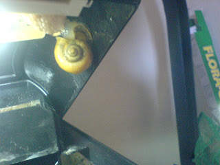
We have two apple snails (sold as an "ivory mystery snail" and a "golden mystery snail") in our small 6 gallon Eclipse tank. Evidently, the golden snail is a female and the ivory snail is a male, and so they mate all the time. In most tanks, this isn't a problem because the amphibious apple snails have to leave the water to lay their eggs and they can't do that when the tank has a lid on it. However, the Eclipse tank has a large dome-shaped lid so that everything (pump, filter, etc.) can be built into it. So, our female has been crawling up into the lid and laying eggs.

This morning, I couldn't find the female in the bottom part of the tank, and so I lifted the lid... and there she was! I've never seen pictures of an apple snail LAYING eggs, so I thought I'd take some. Unfortunately, they came out kinda blurry, but at least it's something!
You can see the egg sac she's laying right next to her. You can see that as she moves backward, the egg sac gets longer.

In the first picture, on another part of the lid, are some of the remnants of an old egg sac that has hatched (before we realized she was leaving the tank to lay her eggs).

Anyone have any ideas about how to prevent the snails from leaving the water? (note: throwing away the tank is not an option) We'd move the snails to our big tank that has a flat lid, but we're pretty sure our freshwater puffer would slowly dine on the snails until they died a long slow death.