Showing posts with label mathematics. Show all posts

Saturday, April 20, 2019

Stochastic versus random: The difference is whether you're describing a model or a focal system


It seems like there is a lot of confusion in quantitative modeling circles over the relationship between "randomness" and "stochasticity." This is in large part because the success of stochastic models to make sense of the world around us has led to wide use of stochastic modeling, so much that "stochastic" has become a near synonym for "random." However, the two terms are not identical.

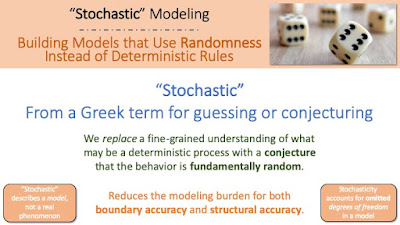
Stochastic modeling summary slide from SOS 212 (Systems, Dynamics, and Sustainability), an introductory modeling course taught by Theodore (Ted) Pavlic at Arizona State University
Slide from SOS 212 (Systems, Dynamics, and Sustainability), an introductory modeling course I teach

"Randomness" is a general term representing a special kind of uncertainty where the frequency of possible outcomes can be described using probabilistic methods. Where a photon is going to be at a particular instant of time is fundamentally random; it can only be described using a probability distribution. There are some kinds of uncertainty that cannot be described probabilistically. For example, I might know that an experiment can end in one of three different ways, but exactly how it will end depends upon which participant is performing the experiment. If I need to describe how the experiment can end but do not have any ability to specify a probabilistic weighting of the outcomes, I can describe the system as having a non-deterministic outcome. So something can be fundamentally random or non-deterministic. If it's random, you have some way to describe how one outcome might be more likely than another.

"Stochastic" is a term originating from Greek for "guess" or "conjecture." It describes a modeling technique to simplify a model by assuming (guessing/conjecturing) that the system being modeled is random, even if it is not. In other words, rather than having to account for a wide range of degrees of freedom that might be necessary to specify how a system is going to evolve, you substitute all of that detailed deterministic modeling with a crude approximation of the outcome being "random". The modeling burden then shifts from getting everything right down to high levels of precision to shaping the probability distributions to best match the outcomes that are most likely, regardless of what the underlying mechanism is. So a "stochastic model" is one that describes a system using randomness regardless of whether there is any reason to believe that the randomness is fundamental. It is a modeling trick to add analytically tractability to models that would otherwise be prohibitively complex to be useful.

So you shouldn't refer to phenomena themselves as being "stochastic." It is OK to say that the phenomena is random (if you really believe that). Or it is OK to say you use a stochastic model to describe the system (which implies that you will use randomness in order to omit a large number of degrees of freedom, thus making the model "simpler"). But you shouldn't use "stochastic" as a synonym for "random."

Wednesday, April 10, 2019

Bifurcation Diagrams, Hysteresis, and Tipping Points: Explanations Without Math

I teach a system dynamics modeling course (SOS 212: Systems, Dynamics, and Sustainability) at Arizona State University. It is a required course for our Sustainability BS students, which they ideally take in their second year after taking SOS 211, which is essentially Calculus I. The two courses together give them quantitative modeling fundamentals that they hopefully can make use of in other courses downstream and their careers in the future.

I end up having to cover a lot of content in SOS 212 that I myself learned through the lens of mathematics, but these students are learning it much earlier than I did and without many of the mathematical fundamentals. So I have to come up with explanations that do not rely on the mathematics. Here is an example from a recent lecture on bifurcation diagrams, hysteresis, and tipping points. It builds upon a fisheries example (from Morecroft's 2015 textbook) that uses a "Net regeneration" lookup table in lieu of a formal mathematical expression.


You can find additional videos related to this course at my SOS 212: System, Dynamics, and Sustainability playlist.

Thursday, January 24, 2013

Discrete-time Phase Portraits?

I was contacted recently by e-mail asking how to produce a phase portrait of a discrete-time system. In my initial response, I explained that a true "phase portrait" wasn't defined for discrete-time systems because the technical notion of a phase portrait depends on a special structure that comes along with ordinary differential equations. The original poster needed some additional clarification, and so I sent a second e-mail that I have posted below. It touches a little bit on the original poster's question, it comments on differences between discrete-time and continuous-time systems, it talks a bit about chaos, and it gives a brief description of Poincaré/return maps that are often used in the study of approximately periodic systems.

My point is that a discrete-time system really cannot be interpreted within a field-theoretic framework. A "phase portrait" captures both position and momentum of a continuous-time system described by an ordinary differential equation. These momentum variables setup the "field" that gives structure to the phase portrait. In a discrete-time system, we don't have the same kind of momentum.

     For a continuous-time system, I can plot a point at an individual position, and I can also then draw a vector pointing away from that point representing the velocity at that instant of time. It is these velocity vectors that are put together to make a phase portrait of the system.

     For a discrete-time system, there is no point-based velocity. In order for me to calculate the approximate "velocity" at a point, I need to know the position at the next point. Then I can draw a line between those two points and approximate the "velocity" of the system as going from the first point to the second point. However, if I have to know the next point in future anyway, it's more useful to just draw the second point.

     Now, some discrete-time systems have a more predictable structure. For example, if you have a linear time-invariant discrete-time system like:

x[k+1] = M*x[k]

then the algebraic structure of the "M" matrix gives us insight into how trajectories will evolve. So for these special cases, it is possible to draw a kind of "phase portrait" for the discrete-time system. However, this is primarily because such a discrete-time system can be viewed as a sampled version of a continuous-time linear time-invariant system which does have a phase portrait.

     So, for an arbitrary discrete-time system, the best thing you can do is explore trajectories from different initial conditions. Gradually, as you explore the space more and more, you may find boundaries of attractors (possibly strange attractors). A complication with discrete-time systems is that the "next" point may be very far from the "previous" point. Take, for example:

x[k+1] = -1.1*x[k]

If you start at x[0]=1, the trajectory will bounce from point clustered above 1 to points clustered below -1. In a continuous-time system, you might expect to see initial conditions above 1 stay near 1 and initial conditions below -1 stay near -1. That is, in a continuous-time system, you wouldn't imagine trajectories could cross x=0 (which is an equilibrium/fixed-point of this system). However, the discrete-time system can jump wildly from point to point.

     Take, for example, the Henon map you mention. Wolfram's Mathworld has some nice plots:

http://mathworld.wolfram.com/HenonMap.html

The first pair of side-by-side plots are colored "according to the number of iterations required to escape". That is, the plots were generated by starting at several initial conditions and recording the resulting trajectories. Each "iteration" gives the next point from the previous point. For a while, a trajectory will stay around its initial condition. Eventually, it will escape and move away from the region. The regions are colored based on how many iterations (i.e., how many calculations after the initial condition) it took for the trajectory to leave the region.

     The second pair of side-by-side plots show a SINGLE trajectory started at x[0]=0 and y[0]=0. Each point was recorded and gradually a pattern emerged. Notice how in the left plot the two regions appear to be disconnected. If you saw a phase portrait that looked like this in a continuous-time system, you would conclude that initial conditions within one region would not be able to join the other region for this set of parameters. However, this plot was generated from a SINGLE initial condition. So the plot jumps from points in the top left to points in the bottom right and back.

     So that's how you can explore something like the "phase space" for discrete-time systems. You can probe it with different initial conditions. For chaotic systems, you have to be very careful you don't accidentally jump over an interesting region of initial conditions that may have qualitatively different trajectories that follow from them.

     As an aside, I guess it's also worth mentioning that many popular discrete-time chaotic maps are actually Poincaré maps of continuous-time dynamical systems. Poincaré maps have other names, including "return maps." Consider, for example, the planets as they orbit the sun. The actual orbits of the planets in three dimensions looks like a tangled mess when you consider their histories over several cycles around the sun because each orbit is slightly different than the previous orbit (i.e., they aren't entirely planar). However, if you insert a plane perpendicular to their orbits at a single location, each planet pierces the plane at one point every cycle. The resulting shapes that are poked out of that cross section reveal structure in the orbits.

     I hope that helps! --
     Ted

Tuesday, August 23, 2011

The maximum number of matrix dimensions in MATLAB

[ Background: I was asked what the maximum number of matrix dimensions was in MATLAB today. I responded as follows. ]

You are only limited by the amount of memory available and the maximum number of ELEMENTS (as opposed to dimensions) in a matrix. The actual number of dimensions is just a detail about how the memory is indexed. You can reshape any existing matrix to any number of dimensions (I'll give details below). You can only create a new matrix if it abides by the memory and element limits that vary by computer.

To find out the maximum number of elements for a matrix on your computer, use the MATLAB command "computer" (do "help computer" for details). For example:
[~,maxsize,~]=computer
tells me that I can have 2.8147e+14 elements in matrices on my computer. So I better be sure that:
(number of rows)
   × (number of columns)
   × (number of cubes)
   × (number of 4-th dimensional thinggies)
   × (...)
is less than that number.

To find out about memory limits on your system see, the command "memory" ("help memory" or "doc memory"). Unfortunately, memory may not be available on your system. Alternatively, you can see:

http://www.mathworks.com/support/tech-notes/1100/1110.html

for information about memory limits in MATLAB. For information about the maximum number of elements (and the command "computer" that I discussed above), see (UPDATE: MATLAB has moved this page, and this link doesn't land in the right spot anymore):

http://www.mathworks.com/support/tech-notes/1200/1207.html#15

Regarding dimensions, you can use the command "reshape" to re-index any existing matrix. For example, if I start with the column vector:
A=ones(100,1)
I can turn it into a row vector:
newA = reshape(A, 1, 100)
or a matrix of any number of dimensions so long as the number of elements is still 100.
newA = reshape( A, 2, 2, 25 )
newA = reshape( A, 1, 1, 1, 1, 1, 1, 1, 1, 1, 100, 1 )
newA = reshape( A, 1, 1, 1, 2, 1, 50, 1, 1, 1, 1, 1, 1, 1, 1 )
% etc.
Now, I'm assuming you're using regular MATLAB matrices. Alternatively, you can use sparse matrices so long as you limit yourself to functions that work with sparse matrices:
help sparfun
A sparse matrix stores an index with every element. That lets it "skip over" the 0 elements of the matrix. Consequently, you can store VERY large matrices with an abstract number of elements far larger than anything you can work with in MATLAB... however, most of those abstract elements will be 0.

Thursday, July 07, 2011

Someone asked me about Hilbert transforming minimum-phase magnitude responses today...

Someone sent me this e-mail today:
Thank you for contributing to the Wikipedia article about minimum phase. I gather from the article that I should be able to use the Hilbert transform to compute a phase response from the amplitude response of a minimum phase system. Yet when I compute (in Matlab) the Hilbert transform of the log of the amplitude response of a Butterworth filter (sampled at uniform frequency intervals), the result is not real and does not resemble the phase response of a Butterworth at all. I expected that it would equal the phase response of a Butterworth since a Butterworth is minimum phase. What have I missed? Thank you.
So I responded in an e-mail, and I've pasted that e-mail here.
Assuming that you are using a high-order filter, are you unwrapping your phase? See the MATLAB function "unwrap" for details. Another easy fix is to ensure you're using the NATURAL log to extract the exponent of the magnitude as an exponential. In MATLAB, "log" is natural log and "log10" is common log.

If you still have the problem, make sure your filter is truly minimum
phase. In particular, the transfer function and its inverse must be
stable and CAUSAL. The causality condition is redundant so long as your
notion of stability includes poles induced from unmatched zeros. For
example, the discrete-time filter:
z + 0.5
is not causal and thus has a pole at infinity. So it does not meet the criteria for being minimum phase. On the other hand, the filter:
(z+0.5)/z
is minimum phase. So let's take its impulse response. In MATLAB, you could try:
h = impulse(tf( [1,0.5], [1,0], 0.1));
or...
z = tf('z');
h=impulse( (z+0.5)/z );
or just read it from the numerator and add as many zeros as you'd like...
h=[1,0.5,0,0,0,0,0,0,0,0,0,0,0,0,0,0,0,0,0,0,0];
Then use the FFT:
H=fft(h);
Then use the discrete-time Hilbert transform of the NATURAL log:
X=hilbert(log(abs(H)));
Then, to compare, use "plot":
plot( 1:length(h), -imag(X)*180/pi, 'o', ...
      1:length(h), angle(H)*180/pi, 'x' )
I think you'll find that each x is circled.

To summarize:
h=[1,0.5,0,0,0,0,0,0,0,0,0,0,0,0,0,0,0,0,0,0,0];
H=fft(h);
X=hilbert(log(abs(H)));
plot( 1:length(h), -imag(X)*180/pi, 'o', ...
      1:length(h), angle(H)*180/pi, 'x' )
Here's another interesting case that won't match as well because of the discrete-time approximation.
z = tf('z',1);
H = (z + 0.5)/(z);
[mag,phase,w]=bode(H);
mag=mag(:); phase=phase(:); w=w(:);
X=hilbert(log(mag));
plot(w/pi,-imag(X)*180/pi,w/pi,phase)
As you can see, these two match pretty well in the interior region. You can make some interesting observations about the edges where they don't match well.

Friday, May 06, 2011

Someone asked me to explain the Price equation today...

I got an e-mail today asking for help understanding the Price equation, prompted partly by the recent RadioLab about George Price. The person who e-mailed me made it sound like he was OK with a long explanation, just so long as it explained the ugliness of the mathematics. Here is my response... (pardon the e-mail-esque formatting... I'm just pasting it rather than re-formatting it)

[ This post can also be found on my web page. ]
You shouldn't believe everything the media tells you about the complexity of the Price equation. I'm always frustrated when I hear someone on the radio read the Price equation out loud as a mathematical statement. It is not meant to be a mathematical statement. It is just a logical justification for something we all think should be true -- traits with higher differential fitness advantage should spread throughout a population (which is a critical aspect of natural selection). Price formalized that statement and then proved that the formalism is a tautology. That's all that's important.

It is a very simple idea, and it has almost nothing to do with statistics (because there are no random variables nor data in the price equation). The Price equation is a theoretical statement about the relationship between two sequential generations of a model population. You can use it to predict how the representation of a particular trait will change over time and eventually settle at some fixed distribution. However, again, numerical applications aside, it really is just a mathematical verification of something which makes intuitive sense.

Just to get comfortable with the notation, consider a trait like "height" across a population of n=100 individuals. Each individual might have a different height. Let's say that in our population, people basically have two different heights (perhaps due to sexual dimorphism). So we have two groups:

z_1 = 5 feet
z_2 = 6 feet

We represent the number of people with each height using the variables:

n_1 = 50
n_2 = 50

That is, there are an equal number of 5' tall people and 6' tall people from our 100 person population (note that n_1 + n_2 = n). Further, we find that both 5' tall and 6' tall people tend to have 1 offspring each. That is, they both have an equivalent "fitness" of 1:

w_1 = 1
w_2 = 1

Where w_i is the number of offspring an individual of group i will contribute to the next generation. Let's say we also know that offspring from 5' tall people end up also being 5' tall, and offspring of 6' tall people also end up being 6' tall. Then we have:

z'_1 = 5 feet
z'_2 = 6 feet

So the value of the trait (height) does not change from generation to generation.

Everything above is a parameter of the model. It represents what we know about "height" of individuals in this generation as well as the relationship between the height of an INDIVIDUAL and its offspring. What Price equation does is tell us about how the distribution of height in the POPULATION will change from this generation to the next. It might be helpful to think about Price equation as relating the AVERAGE value of a trait (e.g., height) in one generation to the AVERAGE value of the trait (e.g., height) in the next generation.

So now let's add-on the Price equation stuff. To account for the changes in the average value of the trait (height here), we have to worry about two effects -- "background bias [due to individuals]" (my term) and "differential fitness" (a quantity that drives natural selection):

1.) Imagine that 5' tall parents produced 5' tall offspring (so z'_1=z_1=5 feet, as above), but 6' tall parents produced 10' tall offspring (so z'_2=10 feet in this hypothetical scenario). Then even without worrying about "differential fitness", we might expect an upward shift in AVERAGE height from the parent generation to the offspring generation. This "background bias [due to individuals]" is related to the "E(w_i \delta z_i)" term in the Price equation. It represents the change in a trait at the individual level. I'll give more info about the math later.

2.) Now, instead, assume that z'_1=z_1 and z'_2=z_2 (so offspring height is the same as parent height) as above. It may still be the case that the average height in the offspring generation changes from the parent generation. This would occur if one height had a higher fitness than the other height. Here, we see that w_1=w_2=1. They both have the same fitness, and so we don't expect any differences IN REPRESENTATION from one generation to the other. Note that if w_1=w_2=5, then each individual would produce 5 offspring. Consequently, the TOTAL population would grow, but the DISTRIBUTION of height would stay the same. To make things more interesting, imagine that w_1=1 and w_2=2. Now each 5' tall person produces one 5' tall offspring, but a 6' tall person produces TWO 6' tall offspring. Consequently, the distribution of height would change from parent to offspring generation. The AVERAGE height would shift toward 6' tall people. The "cov(w_i, z_i)" term aggregates this change. It relates the "differential fitness" of one height to its success into growing the representation of that height in the next generation. I'll give more info about the math in a bit. [NOTE that the average fitness represents the average "background" rate of growth from population to population.]

To get ready for an explanation of the actual Price equation, let's get some terminology out of the way.

First, we define the "expectation" or "average" height in the current population with:

E(z_i) = ( n_1 * z_1 + n_2 * z_2 + ... )/n

That is, "E(z_i)" is the average value of the trait (height above). There are n_1 individuals with z_1 value of the trait, and so we have to multiply n_1 * z_1 to get the total contribution of that value of the trait. We do that for each group. We can do the same for other variables too. For example, here's average fitness:

E(w_i) = ( n_1 * w_1 + n_2 * w_2 + ... )/n

The average fitness "E(w_i)" somehow represents the average rate of population growth. If every w_i is 1, then there will be 1-to-1 replacement of parent by offspring and there will be no population growth; likewise, the average "E(w_i)" will be 1 reflecting no growth. However, if every w_i is 5, then "E(w_i)" will also be 5 and the population will grow 5 fold every generation. With some simple arithmetic, it is easy to verify that the total population in the NEXT (i.e., offspring) generation is given by the product of the number of individuals in this generation (n) and the average fitness (E(w_i)).

We can also find the average value of the trait in the NEXT (i.e., offspring) generation. To do so, we have to scale each value of the trait in the next generation (z'_i) by the number of individuals with that trait in the next generation (n_i w_i), and then we have to divide by the total number of individuals in the next generation (n*E(w_i)). So the average value of the trait in the NEXT (i.e., offspring) generation is:

E(z'_i) = ( n_1 * w_1 * z'_1 + n_2 * w_2 * z'_2 + ... )/(n * E(w_i))

For simplicity, let's use symbols "z", "w", and "z'" as a shorthand for those three quantities above. That is:

z = E(z_i)
w = E(w_i)
z' = E(z'_i)

Penultimately, let's define "delta" which gives the difference in a variable from the this generation to the next. The difference in the average value of the trait is:

delta(z) = E(z') - E(z)

that difference may be due either to differential fitness (i.e., when w_i is not the same as w) or to intrinsic height changes at the individual level. Those intrinsic height changes at the individual level are:

delta(z_1) = z'_1 - z_1
delta(z_2) = z'_2 - z_2
...

Finally, let's define this "covariance" formula. For each group i, let's say we have variables A_i and B_i (e.g., z_i and w_i). Let A be the average value of A_i across the population:

A = ( n_1 A_1 + n_2 A_2 + ... )/n

and B be the similarly defined average value of B_i across the population. Then we can define the covariance across the POPULATION in a similar way as we defined average. That is:

cov( A_i, B_i )
=
E( (A_i-A)*(B_i-B) )
=
( n_1*(A_i - A)*(B_i - B) + n_2*(A_2 - A)*(B_2 - B) + ... )/n

That is, cov(A_i,B_i) is the AVERAGE value of the product of the difference between each A_i and its average A and the difference between each B_i and its average B. We call this the "covariance" because:

* If A_i doesn't vary across values of i, then A_i=A (no "variance" in A) so there is no "covariance"

* If B_i doesn't vary, then there is similarly no covariance

* If whenever A_i is far from its average B_i is close to its average, then there is LOW (i.e., near zero) covariance. That is, both A_i and B_i vary across the population, but they don't vary in the same way.

* If whenever A_i is far from its average B_i is also far from its average, then there is HIGH (i.e., far from zero) covariance. Both A_i and B_i vary across the population, and they vary in the same way.

Note that HIGH covariance could be very positive or very negative. In the positive case, A_i and B_i have a similar pattern across values of i. In the negative case, A_i and B_i have mirrored patterns across values of i (i.e., A_i is very positive when B_i is very negative and vice versa). LOW covariance is specifically when the cov() formula is near zero. That indicates that the pattern of A_i has little relationship to the pattern of B_i.

Now, let's look at the Price equation more closely. The left-hand side:

w*delta(z)

is roughly the amount of new trait ADDED to each "average" individual. So if the average trait shifts (e.g., from 5.5' tall to 6.5' tall, corresponding to a delta(z) of 1'), but the population has GROWN as well (i.e., "w>1"), then amount of height "added" to the parent population to get the offspring population is more than just 1' per person. We scale the 1' per person by the "w" growth rate. Thus, "w delta(z)" captures effects of population growth (which naturally adds trait to a population) and mean change in representation. Note that if the AVERAGE trait did not change ("delta(z)=0") but the population did grow ("w>1"), then we interpret "w delta(z)=0" to mean that even though the "total amount" of trait increased due to population increase, there was no marginal change in each individual's trait (i.e., individuals aren't getting taller; the population is just getting larger).

Now let's look at the right-hand side:

cov(w_i, z_i) + E(w_i*delta(z_i))

This implies that the amount of new trait added to each average individual is the combination of two components.

To parallel the discussion above, let's consider the E() part first:

E(w_i * delta(z_i))

we can expand this average to be:

( n_1*w_1*(z'_1 - z_1) + n_2*w_2*(z'_2 - z_2) + ... )/n

That is, delta(z_i) gives us the average change from AN INDIVIDUAL to A SINGLE OFFSPRING from z_i to z_i'. The w_i part ACCUMULATES those changes to EACH offspring. For example, if w_1=2, then group 1 parents have 2 offspring. So the total increase in the trait from group 1 is not delta(z_1) but is 2*delta(z_1). So you can see how this is the "BACKGROUND BIAS" representing the "w*delta(z)" component that we get even without worrying about differential fitness. This represents the change in "w*delta(z)" just due to INDIVIDUALS and POPULATION GROWTH.

Next, look at the covariance:

cov(w_i, z_i)

The covariance of w_i and z_i is a measure of how much the DIFFERENTIAL FITNESS contributes to added trait. Recall the formula for cov(w_i,z_i):

E( (w_i-w)*(z_i-z) )

which is equivalent to:

( n_1*(w_1-w)*(z_1-z) + n_2*(w_2-w)*(z_2-z) + ... )/n

Here, the quantity (w_i-w) is the "differential fitness" of group i, and the quantity (z_i-z) represents the location of the trait with respect to the average trait. So:

* if the fitness varies in a similar way as the level of trait across values of i, then the average value of the trait will tend to increase from population to population

* if the fitness varies in exactly the opposite way as the level of the trait across values of i, then the average value of the trait will tend to decrease from population to population

* if the fitness varies differently than the level of the trait, then there will be little change in the average trait from population to population

* if there is no variance in either fitness nor level of the trait, there will be little change in the average trait

Put in other words:

* if high differential fitness always comes with high values of the trait and low differential fitness always comes with low values of the trait, then there will be selection toward MORE trait

* if high differential fitness always comes with to low values of the trait and low differential fitness always comes with high values of the trait, then there will be selection toward LESS trait

* if differential fitness variation has no relationship to trait level variation, then selection will not change the average value of the trait

* if there is no variation in the trait or no variation in the fitness, then selection will not change the average value of the trait

Put in MORE words at a more individual group level:

If a group i has both a high "differential fitness" (w_i-w) AND a high (z_i-z), then its FITNESS w_i is far above the average fitness w and its level of the trait z_i is far above the average value of the trait z. Either one of those alone would be enough to cause the "total amount" of trait to shift upward. On the other hand, if BOTH (w_i-w) and (z_i-z) are NEGATIVE, then the average population is already far away from this trait value AND has a much higher fitness. Consequently, the motion of the average trait will still be upward, but here upward is AWAY from the trait z_i (because z_i is under the average z). Finally, if (w_i-w) and (z_i-z) have opposite signs, the motion of the average trait z will be negative, which will either be heading toward z_i if w_i>w or away from z_i if w_i<w. The covariance formula takes the average value of (w_i-w)(z_i-z). That average represents the contribution to the amount of trait "added" to each individual due to DIFFERENTIAL FITNESS.

So there you have it. Assuming that "w" (average fitness -- which is a growth rate) is not zero (which just assumes that the population does not die out in one generation), then we can divide everything by "w" to get a less complicated (but equivalent) Price equation:

delta(z) = ( cov(w_i,z_i) + E(w_i*delta(z_i)) )/w

So now we have an equation representing the average change from parent to offspring population. If you expand all the formulas, you can verify that this statement is equivalent to:

delta(z) = cov(w_i/w, z_i) + E( (w_i/w)*delta(z_i) )

The quotient "w_i/w" is a "fractional fitness." It is a measure comparing the fitness of group i with the average fitness, where high differential fitness corresponds to w_i/w > 1 and low differential fitness corresponds to w_i/w < 1. So let's create a new variable

v_i = w_i/w

to be the fractional fitness. Then we can rewrite Price's equation to be:

delta(z) = cov( v_i, z_i ) + E( v_i*delta(z_i) )

This version gets rid of the need to worry about scaling for population growth. If you think about it, v_i is just a normalized version of w_i where you have "factored out" the background growth rate of the population. So now we basically have:

AVERAGE_CHANGE
=
POPULATION_CHANGE_DUE_TO_DIFFERENTIAL_FITNESS
+
POPULATION_CHANGE_DUE_TO_INDIVIDUAL_CHANGES

In other words:

"the change in the average value of the trait is due to two parts:

1. The differential fitness of each value represented in the population

2. The individual change from parent trait level to offspring trait level"

So if you wish to go back to the "height" example...

"The average height increases when:
1. Natural selection favors increases in height
OR
2. Tall people have taller offspring"

You could create other variations that work as well:

"The average height DEcreases when:
1. Natural selection favors DEcreases in height
OR
2. Short people have shorter offspring"

====

"The average height stays the same when:
1. Natural selection has no preference for height
AND
2. Short people have short offspring and tall people have tall offspring"

====

"The average height DEcreases when:
1. Natural selection has no preference for height
AND
2. Short people have short offspring and tall people have short offspring"

====

"The average height INcreases when:
1. Natural selection has no preference for height
AND
2. Short people have tall offspring and tall people have tall offspring"

Monday, March 07, 2011

MATLAB script to prove to you that the perfect squares are the switches that are toggled

Evidently, this problem exists in both "switch" and "locker" forms. Assume that there are 100 switches are initially off and numbered from 1 to 100.
  • First, you toggle multiples of 1 (i.e., every switch gets turned on),
  • and then you toggle multiples of 2 (i.e., every even-numbered switch gets turned off),
  • and then you toggle multiples of 3 (i.e., switches 3, 6, 9, 12, ... are toggled),
  • ...
  • and then you toggle multiples of 99 (i.e., switch 99 is toggled),
  • and then you toggle multiples of 100 (i.e., switch 100 is toggled).
After this process, which switches are "on"?

Examining the problem, you notice that switches are toggled the same number of times as they have unique factors. For example, switch 6 is toggled 4 times, which corresponds to its unique factors, 1, 2, 3, and 6. However, switch 4 is toggled only 3 times, which corresponds to its unique factors, 1, 2, and 4 (i.e., even though 4 = 2 × 2, the factor 2 is only represented in the list once because it is duplicated). Moreover, it is only the perfect squares (1, 4, 9, 16, 25, 36, 49, 64, 81, 100) that will have repeated factors (i.e., their whole square roots), and so it is only those switches that will be flipped and odd number of times. Furthermore, it is only those switches that will be "on" after this game.

To verify this to yourself, use a MATLAB script:
% All switches initially off
switches = zeros(1,100);

% Toggle multiples of the current switch, including the current switch
for i = 1:100
% These are the switches to toggle
ivec = i:i:100;

% xor'ing them with 1's toggles them
switches(ivec) = bitxor(switches(ivec), 1);
end

% Show the indexes of the switches that are "on" after this process
% (expect perfect squares: 1 4 9 16 25 36 49 64 81 100)
find( switches )
Running the script results in:
ans =

1     4     9    16    25    36    49    64    81   100
which is what we expected.

Of course, you could also keep track of how many times you made a flip. XOR can help with this too.
% All switches initially off
switches = zeros(1,100);
new_switches = zeros(1,100);
num_flips = zeros(1,100);

% Toggle multiples of the current switch, including the current switch
% (gratuitous use of bitxor as a demo)
for i = 1:100
% These are the switches to toggle
ivec = i:i:100;

% xor'ing them with 1's toggles them
new_switches(ivec) = bitxor(switches(ivec), 1);

% count the flips
% ( num_flips(ivec) = num_flips(ivec)+1  works too)
num_flips = num_flips + bitxor( new_switches, switches );

% commit new_switches to switches to maintain invariant
% (can omit new_switches by not using second bitxor above)
switches = new_switches;
end

% Show the indexes of the switches that are "on" after this process
% (expect perfect squares: 1 4 9 16 25 36 49 64 81 100)
find( switches )
Then, from the console, we can issue commands like:
num_flips( find(switches) )     % shows number of flips for switches ending "on"
num_flips( find(switches==0) )  % shows number of flips for switches ending "off"
find( mod(num_flips,2)==1 )     % verifies odd-count flips have perfect-square indexes
So that's fun.

Friday, February 18, 2011

Dr. Bernoulli gets a job: Mathematics of the Job Search – Faculty Version

I recently found out that the Duke Computer Science department had 404 applicants for the open position in their department. I mentioned that to a CS professor from a different university, and he didn't seem surprised by that number. Moreover, when you think about how many "faculty candidate" lectures there usually are within a CS-like department each hiring season, and you consider that those interviewees are likely a small selection of the total applicants, then 404 starts sounding reasonable.

When there are 404 applicants who each have PhD degrees, publications, and possible post-doctoral or existing faculty appointments, let's also assume that the objective function that each department is maximizing is pretty flat. If you don't like that assumption, then assume we have no prior information, and so we will maximize entropy and assume that each applicant has a 1/404 chance of being picked for the job (in reality, this probability is itself conditioned on whether the state steps in and has a hiring freeze... so the real probability might be closer to 1/1000). So that is a very low number. Can we fight low probability with high volume of applications?

Assume we apply to N schools where the probability of getting an offer is
p = 1/404
at each of them. Then the probability of not getting an offer from each of them is
1 - p = 403/404,
and so the probability of not getting an offer from all of them is
(1 - p)N = (403/404)N.
So finally we arrive at the probability of getting an offer from at least one of them, which is
1 - (1 - p)N = 1 - (403/404)N.
Hypothetically speaking, let's say you apply to N = 50 such positions. Then you have a
1 - (403/404)N = 1 - (403/404)50 ≈ 11.65%
probability of getting the offer. Of course, if you were paying attention, you remember that p (1/404) is very small in this example. Consequently, the (1 - (1 - p)N) curve looks linear for a wide region around the origin. So even though you remember your fourth-grade math teacher teaching you that you cannot additively accumulate probabilities (i.e., your probability of getting a job is not (N × p)), in this small-p case, it is a pretty decent approximation. In particular, even with our ostensibly large N, it is the case that
N × p = (50)(1/404) ≈ 12.38%,
which is pretty close to our slightly more dismal 11.65%.

In December, I ran into a woman who just got finished submitting all of her faculty positions. She said she applying to just 10 of them because she was exhausted and figured she was just practicing this round. Setting N = 10 reduces your chances to 2.45%. Having said that, the distribution across the applicant pool is certainly not flat. Her home institution, research, adviser, and other factors make her a very attractive candidate who will likely do well with such a low N... In fact, she was recently interviewed at a university near me (that, again, may have to deal with hiring freezes, etc., in the near future).

Now, in my case... Maybe I should burn my CV and dust off my résumé... I hope I'm not too old and outdated.